WP107: Using CFD for Data Center Design and Analysis

Introduction

Computational fluid dynamics (CFD) is the numerical simulation of fluid flow. It predicts velocities, temperatures and other quantities across a wide range of applications: the air over an aircraft wing, the water past a ship’s hull, the mixing of two liquids in a tank. It is routinely used to model the flow inside buildings, and this paper covers one kind of room: data centers. In a data center, CFD predicts where the cold supply air goes, where the hot exhaust goes, and what temperature each rack takes in.

This paper is a new edition of WP107, first published in 2011. It explains how a CFD model of a data center is built, solved and read, and works each step through one room, the one studied in WP110 [2], WP111 [3] and WP112 [4]. It then covers how data center equipment is represented in a model, what to include, and practices that avoid common problems.

The Example Room

The room is 124 ft by 57.5 ft, with 234 racks at 4 kW each, 936 kW in total, in seven enclosed hot aisle pairs (Figure 1). Eighteen cooling units line the two long walls. Each supplies about 6,500 CFM, 117,000 CFM in total, and the racks draw about 114,300 CFM. The room has a slab floor, with no raised floor, and an 11.75 ft ceiling with a 21 in. return plenum above it. Each hot aisle is enclosed, and its exhaust leaves through grilles into the ceiling plenum, which carries it back to the cooling units.

The case used throughout is one from WP112: the supply air raised from 60°F to 64°F, with one unit 5°F warmer than the rest, as built. At that temperature a few racks are close to the ASHRAE recommended limit for inlet air, 80.6°F [1], which makes it a good case for showing what a converged solution does and does not settle. It was built and solved with CoolSim’s standard model setup, the same one used for customer jobs.

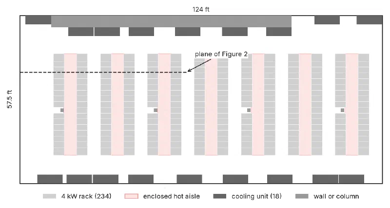
Plan view of the 124 ft by 57.5 ft room: seven pairs of rack rows, each pair enclosing a hot aisle, with cooling units along the upper and lower walls, and a dashed line crossing the first three row pairs marking the plane of Figure 2 — Figure 1
The example room: 234 racks at 4 kW in seven enclosed hot aisle pairs, and 18 cooling units along the long walls. The dashed line marks the vertical plane shown in Figure 2

Computational Fluid Dynamics

The goal of a CFD calculation is to predict the detailed flow field in a region of interest. That means not only the motion of the fluid but also the distribution of its temperature and of anything else the flow carries. It can include other effects, such as turbulence, time dependence, chemical reaction, evaporation, melting or freezing. Despite the range of applications, the same general method is used. Conservation equations are solved in small cells that fill the region. The region must therefore be divided into a large number of cells, and the equations rewritten so that they can be solved in each one. The next sections describe those two steps, how the solution is obtained, and how the results are read.

Geometry and Mesh

A CFD simulation begins with the geometry of the problem. The region to be modeled is called the computational domain, and the geometry consists of its boundaries and all the objects inside it. Where computer-aided design (CAD) software describes solid objects, CFD is concerned with the space inside and between them, where the air flows. Data center CFD software provides ready-made objects for cooling units, racks, PDUs, perforated tiles, grilles, containment panels and other common components, which are placed and sized within the room.

The space is then divided into a large number of small cells, where the equations are solved and the results stored. The lines and faces that separate the cells are called the mesh or grid. Cells can be of almost any shape; six-sided hexahedra, five-sided prisms and pyramids, and four-sided tetrahedra are the most common. Making a mesh by hand is slow work, and data center software, CoolSim included, builds it automatically from the objects in the room.

The example room’s mesh has 655,782 cells, all hexahedra on a Cartesian grid, with lines at right angles (Figure 2). The mesh is non-uniform: cells are smaller where the geometry needs more detail, such as at the faces of the racks and the edges of the grilles and containment panels, and larger in open space. In this mesh each line runs across the whole room, so a line placed for one object also crosses parts of the room far from it. The close lines in the cold aisle near 25 ft in Figure 2 are there for the edges of three cooling units along the walls, 12 ft or more from this plane. Around round or angled objects, meshing software can instead bend the cells to fit or switch to another cell shape, which often reduces the number of cells.

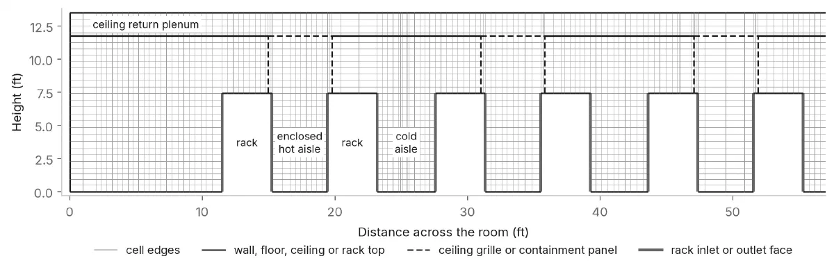
Vertical slice through the mesh across three rack pairs, showing a grid of rectangular cells from the floor to the top of the ceiling plenum, with close-spaced lines at the edges of the racks, grilles and containment panels and in one cold aisle — Figure 2
The mesh on a vertical plane across three rack pairs, at the dashed line in Figure 1. Containment panels close each hot aisle from the rack tops to the ceiling, and ceiling grilles lead from the hot aisle into the return plenum. The inside of a rack is not part of the domain and is not meshed

The Equations

Consider a small volume of moving fluid. It is carried along and rotated by the flow, which is called convection, and it is stretched and twisted by differences in velocity from one side of it to the other, which leads to a process called diffusion. In the simplest case these two processes govern how the fluid changes from one moment to the next. Other effects can also contribute: heat, for example, can make a gas expand and rise. Conservation equations account for convection, diffusion and any sources of the conserved quantity, and together they describe the motion of the fluid. They are coupled: a change in one variable, such as temperature, can change another, such as velocity. In software written for a particular application, such as data center airflow, the user is not expected to control how the equations are solved. It is still worth knowing what they are.

Continuity

The equation of continuity is a statement of mass conservation. Consider fluid of density $\rho$ flowing through the six faces of a small rectangular block with sides of length $\Delta x$ , $\Delta y$ and $\Delta z$ , where the velocity components in the three coordinate directions are $u$ , $v$ and $w$ . For mass to be conserved, the net mass flow through all six faces must be zero:

\rho\left(u_{out}-u_{in}\right)\Delta y \Delta z + \rho\left(v_{out}-v_{in}\right)\Delta x \Delta z + \rho\left(w_{out}-w_{in}\right)\Delta x \Delta y = 0

Dividing through by $\Delta x \Delta y \Delta z$ , the equation can be written as:

\rho\frac{\Delta u}{\Delta x}+\rho\frac{\Delta v}{\Delta y}+\rho\frac{\Delta w}{\Delta z}=0

or, in differential form, for the more general case where the density changes in time ( $t$ ) and space:

\frac{\partial\rho}{\partial t}+\frac{\partial}{\partial x}(\rho u)+\frac{\partial}{\partial y}(\rho v)+\frac{\partial}{\partial z}(\rho w)=0

Momentum

Similar reasoning gives an equation for the conservation of momentum in each of the three coordinate directions. Momentum conservation is more complicated than mass conservation. Pressure differences and gravity act as sources of momentum. Momentum also diffuses, because of differences in velocity within the fluid, as when a jet of air spreads into the still air around it. Taking these effects into account, the momentum equation in the $x$ direction, for a fluid whose density changes little, takes the form:

\rho\left(\frac{\partial u}{\partial t}+u\frac{\partial u}{\partial x}+v\frac{\partial u}{\partial y}+w\frac{\partial u}{\partial z}\right)=-\frac{\partial p}{\partial x}+\mu\left(\frac{\partial^2u}{\partial x^2}+\frac{\partial^2u}{\partial y^2}+\frac{\partial^2u}{\partial z^2}\right)+\rho g_x+F_x

Here $p$ is the pressure, $\mu$ the fluid viscosity, $g$ the acceleration due to gravity, and $F$ any other force present. The term multiplied by $\mu$ is the diffusion term. The three momentum equations, for the $u$ , $v$ and $w$ components of velocity, together with the continuity equation are called the Navier-Stokes equations. They are four equations for four unknowns: the three velocity components and the pressure.

Turbulence

At the air speeds in a data center the flow is turbulent, and the Navier-Stokes equations alone are not enough to describe it in practice. The main effect of turbulence is to increase diffusion: the fluid behaves as if its viscosity were much higher. There are several ways to include this. The simplest adds a turbulent viscosity based on local flow and geometry. More involved approaches solve additional transport equations for the turbulence, and time-dependent calculations can resolve some of its fluctuations directly. Enclosed rooms such as data centers are often modeled with the simpler approaches.

The example uses the simplest. In the momentum equations the viscosity $\mu$ becomes $\mu+\mu_t$ , where the turbulent viscosity $\mu_t$ comes from a mixing-length model: it is computed in each cell from the local velocity gradients and the distance to the nearest wall, and no extra equations are solved.

Energy and Buoyancy

A conservation equation for thermal energy, analogous to those for mass and momentum, carries heat from where the racks add it to where the cooling units remove it. Turbulence increases the diffusion of heat just as it increases the diffusion of momentum.

Temperature also changes the flow. In the example, the density of the air is computed from its temperature with the ideal gas law at a fixed pressure, so warm air is lighter than cool air. Gravity acts straight down, so the gravity term appears in the vertical momentum equation, where it makes the warmer air rise. This is buoyancy, and it is how the energy equation feeds back into the momentum equations.

Solving the Equations

Think of each cell as having a point at its center. The solver’s task is to find a value of every variable, for every equation, at every such point. The example solves five equations, continuity, three momentum equations and energy, in 655,782 cells: about 3.3 million values to find.

The differential equations are converted into algebraic ones, a set for each cell. To measure how well they balance in a cell, the solver needs the values of the variables at the cell’s faces, which it estimates from the values at the cell centers, and numerical methods differ in how they make that estimate. The method, the size and shape of the cells, and the nature of the flow together decide how accurate the solution is.

Residuals and Convergence

The coupled equations cannot be solved exactly, so they are solved iteratively. Roughly speaking, the solver starts from a guess for every variable in every cell, measures how far each equation is from balancing, improves the guess and repeats. The imbalance of one equation, summed over all the cells, is that equation’s residual. The residuals fall as the solution improves, and the solution is called converged once each is below a preset limit. Only results from converged solutions are meaningful.

The top of Figure 3 shows the example’s five residuals, scaled so that each can be compared with a fixed limit. The limits are 10⁻³ for continuity and the three velocities and 10⁻⁶ for energy. All five were met at iteration 200, and the solver stopped there.

Top: the continuity, three velocity and energy residuals falling on a log scale until all are under their limits at iteration 200, then jumping when the case is reopened and settling again by iteration 312. 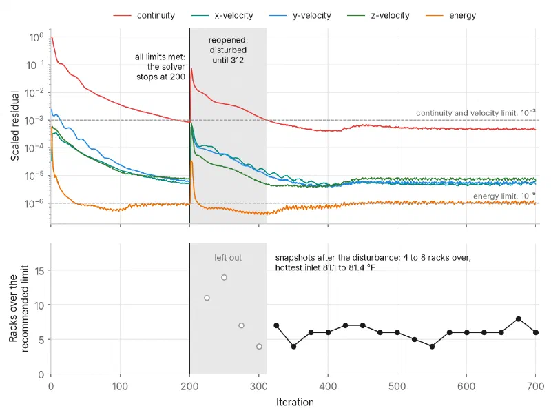Bottom: the number of racks over the ASHRAE recommended limit in snapshots every 25 iterations after 200, with the four taken before 312 shown hollow and the sixteen after it between 4 and 8 — Figure 3
Top: the residuals of the example case. The solver stops at iteration 200, when all five are under their limits; the case is then reopened and run on, which disturbs it until iteration 312 (shaded). Bottom: racks over the ASHRAE recommended limit in a snapshot every 25 iterations. Snapshots taken during the disturbance are left out

How Settled Is a Converged Solution?

Convergence means that the equations balance to within the limits. It does not mean that every number in the room has stopped moving. To see how much the answer moves after convergence, the example case was reopened and run for another 500 iterations, with a snapshot of every rack’s inlet temperature every 25 iterations (Figure 3, bottom).

Reopening a solved case disturbs it. The continuity residual jumped to about 7 × 10⁻² and was not back under its limit until iteration 312. The four snapshots taken in that time, with 4 to 14 racks over the recommended limit, are of a solution the solver would not have accepted, and they are left out.

The 16 snapshots after that show 4 to 8 racks over the recommended limit and a hottest rack inlet of 81.1°F to 81.4°F. Throughout, continuity and the velocities stay under their limit, and energy stays close to its own, never above 1.24 × 10⁻⁶. The hottest inlet moves by only 0.3°F. The count moves more, because several racks sit close to the limit and small changes carry them across it and back.

A CoolSim report is taken at the iteration where the limits are met, so it is one such snapshot. A rack reported just over or just under a limit is best read as being at the limit.

A converged solution is also not necessarily a correct one. Residuals measure how well the equations have been solved, not how well the model represents the room. That is checked by comparing the model with measurements, as described under The Modeling Process below.

Displaying the Results

A converged solution holds values for millions of points. One of the simplest ways to examine it is one plane at a time. A plane can be placed at any position, or on the surface of an object such as the inlet side of a rack row, and used to show contours of a variable or arrows for the velocity. An iso-surface, by contrast, is a surface, usually not flat, on which one variable has a constant value: a surface of constant temperature, for example, colored by some other variable. Pathlines trace the paths of imaginary particles of air released from a surface, such as the supply of a cooling unit or the exhaust of a rack. They can be colored by temperature and animated, and they are often the clearest way to show where hot exhaust ends up.

For a design question, the most direct display is often the answer itself. In Figure 4, each rack is colored by its hottest inlet reading against the ASHRAE limits.

Using CFD to Compare Designs

One of the most important uses of CFD is to compare designs before any equipment is moved. Figure 4 compares the example room as built with the same room with its airflow shifted: the six units at the left end each supply 25% less air and the other twelve 12.5% more, so the total supply is unchanged [4]. As built, five racks toward the right end of the room are over the recommended limit. With the airflow shifted, none are, and the hottest rack inlet falls from 81.1°F–81.4°F to 78.4°F–79.0°F.

A heat and airflow balance cannot tell these two rooms apart. Both have the same heat load, the same total air and the same supply temperature. What differs is where the air goes, and that is what CFD predicts.

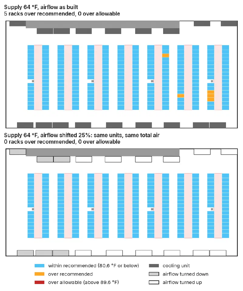
Two plan views of the room at 64 degrees F supply with each rack colored by its hottest inlet reading: as built, five racks toward the right end are over the recommended limit; with the airflow shifted 25%, none are — Figure 4
Each rack colored by its hottest inlet reading, the median of 16 snapshots as built (top) and 15 with the airflow shifted (bottom), at 64°F supply. Units whose airflow was cut are shown in light gray, and units given more air in outline

The Modeling Process

CFD is most useful as a planning tool. An existing room is modeled, the model is compared with measurements, and once the two agree the model is changed to try out a move, an addition or a new layout before anything is done to the room. The same approach is used in the automotive industry to test body shapes before any metal is bent, and it suits data centers, where changes to equipment are routine.

How well this works depends on how accurate the model is, so where measurements are available, compare against them first. Start with a simple model: average heat loads in the racks, small obstructions left out, and a coarse mesh. A comparison with measurements will usually show some discrepancies, and those point to what to add on the next pass. Suppose, for example, that a simple model of a raised-floor room leaves out the small pipes under the floor and gives every rack an average heat load. If the airflow through the floor tiles agrees with measurements but some hot spots in the room are missed, leaving out the pipes was probably acceptable, but averaging the heat loads in the racks was not. The refined model adds that detail, and the comparison is repeated.

More than one round of refinement may be needed. If the model still does not agree after several, look for the cause. Assumed heat loads and flow rates are a common one, especially where equipment has variable-speed fans that the model does not account for. Measurements can also be wrong, so know how accurate they are. Once a model agrees with the measurements, it becomes the base case for trying out changes.

Modeling Data Center Equipment

Each application of CFD has its own common components, and each is represented in a way that suits it. A light, for example, might be modeled as a heat source with the shape of its housing, and a fan as a flat area through which a set flow of air passes. This section covers how the equipment familiar to facilities engineers is represented: cooling units, racks, power equipment, tiles, grilles, containment, and ducts.

Cooling Units

Computer room air conditioners (CRACs) and air handlers (CRAHs) draw in warm air from the room, cool it, and return it. In normal operation each has a fixed airflow and can remove up to a certain amount of heat.

A cooling unit is usually modeled as a block with two faces that move air: a return face that draws air out of the room, and a supply face that returns the same flow, cooled. The inside of the block is not meshed and is not part of the domain. Some units have two or three supply faces and a single return. Alternatively, the inside of the unit can be meshed, with a heat exchanger that removes heat from the air inside it and a single fan on the supply side, modeled with the fan’s performance curve.

In the example room, each unit is a block 8.75 ft by 3 ft against a long wall, reaching the ceiling. Its top face, open to the ceiling plenum, is its return, and its underside, 2.3 ft above the floor, is its supply. Each supplies about 6,500 CFM at its set temperature.

Downflow, Upflow, In-Row and Overhead

Where the return and supply are placed depends on the room and the kind of unit. Raised-floor rooms usually use downflow units, which supply cold air into the plenum under the floor and draw return air in at the top. The cold air enters the room through perforated floor tiles. Where a ceiling plenum carries the return air, these units often extend up to it, so that the warm return air does not mix with the cold supply air in the room. Rooms without a raised floor often use upflow units, which supply cold air from the top and draw return air in near the floor. In-row units sit between racks, draw warm air from the rack exhausts, often from a hot aisle, and supply cold air on the opposite side, next to the rack intakes. Overhead units, mounted on the ceiling or on the racks, act locally in the same way. Whatever the type, a unit can be modeled as a block with return and supply faces carrying matched flows.

Plug Fans

Some units discharge air radially from plug fans that extend below the unit into the underfloor plenum. These can be modeled with a cylindrical fan, whose surface is the wall of a cylinder rather than a flat face. The volume inside the cylinder is not meshed.

How Units Control Temperature

The simplest model supplies air at a set temperature, whatever the load; the example room uses this. Many units instead control the temperature of the air they return, cycling or modulating their cooling to hold it at a thermostat setting. A model can do this by adjusting the heat each unit removes as the solution proceeds, until its return temperature matches the setting:

\dot{Q}=\dot{m}c_p\left(T_R-T_S\right)

where:

$\dot{Q}$ is the rate of heat removal (W)
$\dot{m}$ is the mass flow rate (kg/s)
$c_p$ is the specific heat of air (J/kg-K)
$T_R$ is the return temperature (K)
$T_S$ is the supply temperature (K)

For many units the manufacturer gives cooling capacity as a function of return temperature, and the model can use that in place of a fixed value of $\dot{Q}$ .

Racks

Where cooling units remove heat from the air, racks of equipment add it. Servers are rated by their heat load, and the same relation gives the airflow needed for a given temperature rise across them. For a rise of 20°F, about 160 CFM of air is needed for every kilowatt. The example room’s racks draw 114,300 CFM for 936 kW, about 122 CFM per kilowatt, an average rise of about 26°F.

A rack can be modeled with an average heat load, or as individual pieces of equipment with blanking panels and gaps between them. Either way, the inside of the rack need not be meshed. Instead, a matched pair of faces takes air out of the room at the rack’s inlet and returns the same flow at its outlet, with the rack’s heat added. In the example room, each of the 234 racks is modeled this way, with a 4 kW load. The inside of a rack can be meshed instead, for example to study temperatures inside individual servers under given conditions in the room.

Racks can be modeled with air flowing front to rear, front to top, bottom to top, or side to side, and flow entering the front can be split between the rear and the top. A top exhaust is reasonable for a rack with an average heat load. For a rack modeled as individual servers it is not, because it is hard to say how much of each server’s air leaves through the top.

In raised-floor rooms, cable cutouts under racks let supply air rise from the plenum into the rack inlets. If they matter, model the rack with an average heat load; otherwise the air from the plenum mixes only into the server nearest the floor.

PDUs and UPSs

PDUs and UPSs also produce heat that must be removed. They typically draw cooling air in through the floor or through side grilles and exhaust it through the top. They can be modeled like racks, with a matched pair of faces and heat added between them, or meshed inside with a heat load in their volume, with openings at the bottom and top so that air can rise through them by natural convection.

Perforated Tiles, Ceiling Grilles and Containment

Perforated tiles let cold air from the underfloor plenum into a raised-floor room where it is needed, usually in front of the rack rows. A tile’s partial open area causes a pressure drop, and the tile also straightens the air passing through it. Tiles are therefore usually modeled as a thin porous region with a much lower resistance normal to the floor than across it, so that the air leaving it rises. Cable cutouts in the floor away from the racks are modeled the same way.

Ceiling grilles cause a pressure drop as the air passes into the ceiling plenum, but they do not need to straighten it. They can be modeled as a thin face with a loss coefficient that gives the right pressure drop. The example room has seven, one over each hot aisle.

Containment panels can be modeled the same way, with a much higher loss. In the example room, the panels that close each hot aisle above the racks have a loss over a hundred times that of the grilles, so almost no air passes through them.

Ducts and Diffusers

In some rooms, ductwork carries cold or warm air and releases it through diffusers, which can direct the air straight down or at an angle. The inside of a duct can be meshed and solved, but need not be. If it is not, the air from the units feeding the duct can be assumed well mixed, so that every diffuser supplies the flow-weighted average temperature, and the total flow can be divided among the diffusers in proportion to their area. Equal flow per unit area is a reasonable assumption for diffusers of similar size, but less so for one just after a sharp bend in the duct. Meshing the duct lets the solution find the temperature and flow at each diffuser.

What to Include in a Model

For a CFD model, a data center is a closed space with very little air or heat entering or leaving. All the heat produced in the room must therefore be removed by the cooling units, and the equipment’s airflow is normally supplied by them too. The most important objects to include are those that produce or remove heat and those that move air: every cooling unit, rack, PDU and UPS, and every tile, grille, duct and diffuser.

Next in importance are objects that change where the air goes or how it mixes: containment panels, baffles or turning vanes in the plenum, blockages under the floor, and large objects in the room that neither produce heat nor move air. Solid baffles need care. The air in the model must form a single connected volume, and baffles that close off an office or closet can leave pockets of air cut off from the rest, which the solver may have difficulty with. Block such spaces out with solid objects instead. Overhead and underfloor cable trays can affect the airflow, and whether to include them depends on their size and position.

Small objects matter least, especially in large rooms. Pipes under the floor less than about 3 in. across, tables and chairs, and filing cabinets are usually too small or too few to change the airflow. Small heat sources such as lights and control stations add to the heat load, but usually little compared with the equipment. People who are in the room most of the time, and windows without shading, may be worth including.

Best Practices

Several articles have been written on best practices for CFD modeling, mostly for analysts who control the mesh and the solver. Users of software written for data centers should still keep a few in mind:

Avoid too much detail. Get a general sense of the airflow before adding objects and detail. A CFD model is not a CAD model, where more detail is usually better.
Avoid small gaps. If a cooling unit is 2 in. from a wall, there is probably no need to model the air between them. Move the unit flush against the wall.
Start with a coarse mesh. Move to a finer mesh only after the results make sense.
Avoid disconnected pockets of air. Block out rooms that take no part in the airflow with solid objects.
Read results near a limit as being at the limit. A rack within a fraction of a degree of a limit can be on either side of it from one iteration to the next.
Learn the software and its limits. Take the recommended training before starting.

Most common modeling problems can be avoided this way. CFD software written for data centers can be used successfully by engineers, designers and technicians with a wide range of backgrounds. When choosing a product, consider ease of use, whether it can do what you need, and the technical support available. If rack-level detail will be important, for example, choose a product that models it.

Conclusions

CFD predicts where the air goes in a data center, which a heat and airflow balance cannot. That exposes problems that do not show up in totals, as in the example room, where the same total air leaves five racks over the recommended limit or none, depending on how it is divided among the units. Layout changes can be tried in a model before equipment is moved or replaced, and CFD can show how the cooling load is shared among the units and what happens when one of them fails [3]. A converged solution balances the equations to within set limits, and results near a limit should be read with the small movement that remains in mind.

References

ASHRAE Technical Committee 9.9, Thermal Guidelines for Data Processing Environments, 5th ed., ASHRAE, 2021.
WP110: Adding AI Racks to an Air-Cooled Data Center, CoolSim, 2026.
WP111: Which Cooling Unit Can You Afford to Lose?, CoolSim, 2026.
WP112: How Warm Can the Supply Air Go?, CoolSim, 2026.