WP101: Analysis of the UNH Data Center Using CFD Modeling
Introduction
In the Fall of 2008, Applied Math Modeling Inc., the UNH Data Center, and students from the UNH Mechanical Engineering Program collaborated on a project to improve the design and thermal efficiency of the UNH Data Center. The UNH Data Center is an off-campus facility that consists of approximately 2700 square feet of floor space, divided into three smaller rooms with a common pressurized subfloor plenum. The goal of the project was first to create a mathematical model of the data center thermal environment using the CoolSim CFD (computational fluid dynamics) application, and then to use the model to improve the cooling efficiency of the room, thereby reducing energy consumption and/or allowing more IT capacity using the existing cooling equipment. Temperature and airflow measurements were made in the data center to ensure that the model was accurately predicting the system behavior.
UNH Data Center Layout
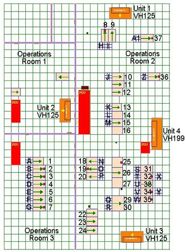
Figure 1
2D floor plan of the UNH Data Center
The existing data center is composed of three main rooms, as shown in Figure 1. The four external walls are considered the domain boundary for the model. This analysis was concerned only with the elements that lie within this boundary, so components such as the HVAC system of the building was not a focus. Instead, attention was centered on how the system dynamics within the rooms can be optimized to achieve a better overall thermal performance. The UNH Data Center is separated into three small rooms labeled Operations Rooms 1, 2, and 3, which are used to house cooling and IT equipment. The design of this data center is a result of the conversion of space once used as a cold storage facility. The partitioning of the data center into separate rooms stems from its original use and poses some unique challenges for cooling.
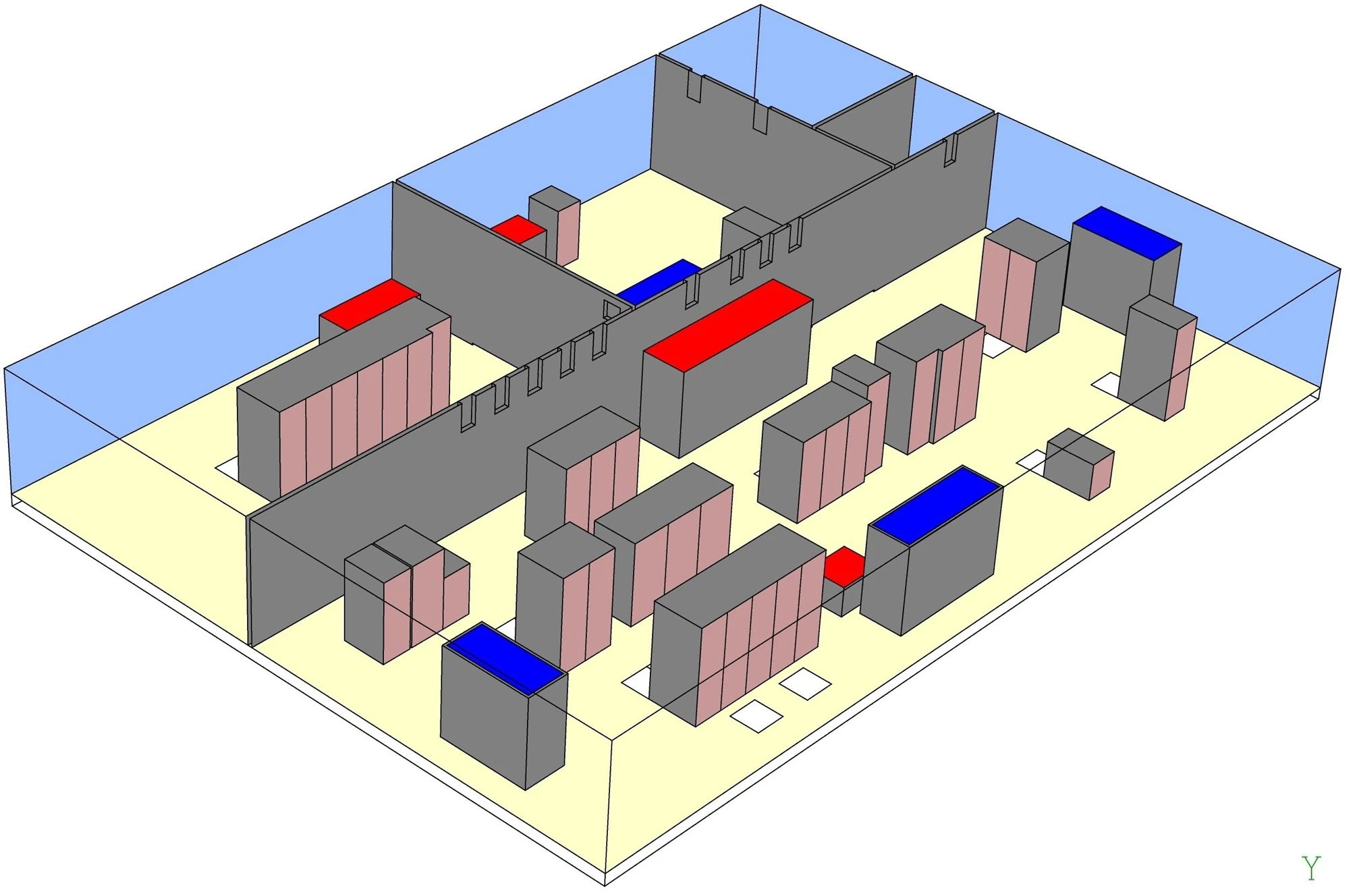
Figure 2
3D model of the UNH Data Center
The main elements in a data center are the racks of servers, power supplies, computer room air conditioning (CRAC) units, and the mechanism for distributing the cold air to the heat-generating components in the room. Here, a raised floor mechanism is used, where cold air from the CRAC units is blown into the subfloor plenum, and perforated tiles are positioned around the equipment to allow the cold air to enter the room and cool the equipment. This data center also utilizes a passive return system, where the heated exhaust air from the racks is allowed to pass freely within the rooms before entering the CRAC returns on top of the cooling units. The perforated tiles are labeled by letter in Figure 1, and the racks by number. A few of the rack numbers are missing. This is due to the fact that the racks are currently empty, but may be populated in future scenarios.
A base model for the data center was created and a simulation was run. The results were used to analyze the flow interactions between the rooms, the effectiveness of the raised floor and existing perforated tile arrangement, the flow paths through and around the servers, and the warm air return to the tops of the air conditioning units.
The UNH data center has a couple of unique characteristics that are important aspects of the existing room configuration. First, the subfloor region is small, with a height of only 9 inches, and a quantity of cable trays and wires in the subfloor reduces the available volume in the plenum and obstructs the flow of supply air in places. Second, the data center was partitioned into smaller rooms for security reasons prior to its current use as a data center. To allow for better performance as a data center, perforated grills were placed in the upper sections of the walls separating the rooms to allow the hot exhaust air to travel freely to the closest CRAC unit.
The data center is cooled by four Liebert CRAC units. Units 1, 3, and 4 are located in Operations Room 2, while Unit 2 is located in Operations Room 1. Table 1 outlines the specifications for each unit. The data center contains 39 server racks. The majority of the racks are located in Operations Room 2. The heat loads for the servers were unknown, so initial estimates were based on worst case specifications supplied by the manufacturer (corresponding to the highest heat loads). The heat loads were then adjusted downward depending on the system configuration. For example, systems configured with half the maximum total memory and CPU cores were modeled at 50% of the manufacturer’s total thermal load.
| Unit | Model | Year | Cooling Capacity (kW) | Flow Rate (CFM) |
|---|---|---|---|---|
| 1 | Liebert DH125 | 2002 | 34.76 | 5650 |
| 2 | Liebert DH125 | 2002 | 34.76 | 5650 |
| 3 | Liebert DH125 | 1999 | 34.76 | 5650 |
| 4 | Liebert FH199 | 1990 | 51.11 | 8400 |
Table 1
CRAC unit specifications
Creating the Model in CoolSim
The methodology for modeling the data center was to first create a model in CoolSim based on the physical characteristics of the room. This process entailed taking inventory of all the equipment types and placements in the room including racks, power supplies, perforated tile locations, walls, under-floor obstructions, cable cutouts, and any other areas where air might be blocked or leak through the raised floor. A baseline CoolSim simulation was then performed to gain insight about the general dynamics of air movement, under floor pressure, and temperature distribution throughout the facility. Care was taken to not make this initial model too complicated in terms of geometry detail, but to include enough detail to obtain the basic flow characteristics. Once the baseline results were calculated, comparisons were made to actual measurements taken in the data center. Based on the comparison between the simulated results and measurements, additional details were added to the model to more closely represent the measured flow characteristics.
Creating the data center in CoolSim was fairly easy and took only about 4 hours. The CoolSim model was built using details of the room geometry, cooling units, rack locations, IT equipment in the racks, and thermal load assumptions for the equipment. All the significant leaks (areas greater than 6 square inches) in the system were also represented in the model. The internal walls separating the rooms included properly positioned vents to allow the flow of return air back to the CRAC units. The vents were assumed to have 40 percent open area.
The most time-consuming aspect of creating the model was acquiring the technical specifications for each piece of IT equipment, required to model the thermal load. Unfortunately, rack electrical load measurements were not feasible in the UNH facility, so load assumptions had to be made using IT manufacturing data. Once the locations and technical specifications for all of the equipment were collected, an average load per rack and corresponding rack flow rate were calculated and input into the software. Based on an assumed 20°F temperature rise across each rack, the flow rate was computed by CoolSim to be 156 CFM/kW of thermal load.
A Data Center Assessment Report, available in the software to provide global totals of heat loads, cooling capacities, and flow rates was used to summarize the equipment in the room. The report is shown in Figure 3. According to this summary, the CRACs provide 49% more cooling capacity and 71% more air flow than is required by the current racks due to the recent retirement of older IT servers. Since one of the CRACs is almost twenty years old and another is ten years old, it is likely that they are not operating at their maximum rated values. The surplus of cooling capacity may therefore be an overestimate if some of the units are operating at a lower performance level. This will be discussed in a later section when the measured rack temperatures are compared to the simulation results. Note, however, that the assessment report is simply a summary and does not take the flow and temperature distribution into account. A CFD simulation is required to predict these distributions, so will provide a far more accurate representation of whether or not the CRACs can adequately cool the equipment, even if some are running at less than peak capacity.
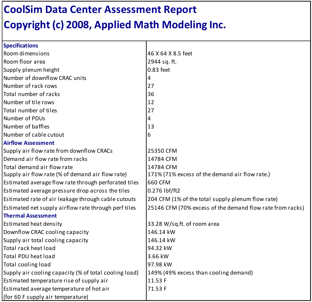
Figure 3
Figure 3: The CoolSim Data Center Assessment Report
Modeling Assumptions
A number of assumptions were made for the creation of the base model. First, because it was not possible to make actual load measurements on each equipment rack in the facility, the maximum rack thermal load was determined by researching the technical specifications for each server and summed for each rack. By comparing the actual configurations in the racks (based on server usage) with the maximum published configurations, an assumption was made that the actual racks were producing 60% of the maximum published heat loads.
Second, an approximation was made in the base model regarding the room geometry. In this model, it was assumed that the subfloor was entirely clear of obstructions such as wires and pipes. This approximation was subsequently dropped because it yielded poor agreement with measurements of flow distribution through the perforated floor tiles. This point will be discussed in a later section.
Third, the cooling capacity for each CRAC unit was based on technical specifications obtained from the manufacturer. The CoolSim software contains a library of DataAire and Liebert CRACs, so that the user can select the make and model number from the list and have all the specifications automatically supplied. This option assumes that the units are operating at the manufacturer’s rated performance levels, which may decline over time due to age. In addition to creating a model using the manufacturer’s cooling capacities, a model was run with reduced cooling capacities, where the reductions were proportional to the age of the unit.
Experimental Measurements
Over 200 measurements were taken in the data center to provide insight into the system behavior. Measurements of airflow and temperature in the data center were done using a Mannix hand-held Air Master WDCFM8951 device. Flow rate measurements where determined by measuring the average air velocity approximately 6 inches above the perforated tile. Measurements were made at roughly 5 positions on each tile - in the center and at each of the corners - and the average velocity was then multiplied by the area of the floor tile to obtain the volumetric flow rate. This method is not nearly as accurate as when a hooded device such as a Velometer is used, but it does represent what most data centers would have available. Velocity measurements were also taken at three different heights for each of the racks and averaged for comparison to simulated data. The Air Master 8951 was also used for temperature measurements, which were made at three points on rack inlets and exits, and then averaged for comparison to the simulated values.
Due to time constraints and instrument limitations, the measurements were sparse. Ideally, a meshing scheme could have been constructed to gather many data points for each measurement, so that accurate averages could be found, and random data points could be discarded. However, this approach was not practical due to the time sensitivity of the project. Furthermore, the goal of taking measurements was to obtain a general idea of the system behavior, and ensure that the model was representative. Therefore, the exactness of the data was less of a priority than the general trending patterns.
Simulation Results and Model Validation
Once the model was complete, a baseline simulation was run, and the results were compared to measurements taken in the data center. A systematic analysis was performed to achieve correlation between the model and the actual system. First, the total air flow predicted by the simulation was compared to the total measured air flow. In Table 2, a comparison between the total measured and simulated flow rates shows very good agreement, with an error of just under 5%. The fact that the simulation does not overpredict the measured airflow suggests that the CRAC flow rates have not declined from their rated values with age.
| Simulated Flow Rate (CFM) | Measured Flow Rate (CFM) | Error (%) |
|---|---|---|
| 25,350 | 26,441 | 5 |
Table 2
Comparison of simulated and measured total air flow rate in the room
The next comparison was of the distribution of air flow through the perforated floor tiles. Figure 4 illustrates the CoolSim baseline results for flow rate along with the measured data. As can be seen, the simulated and measured values for most of the perforated tiles are not in very good agreement, with error that ranges from less than 1% to about 60%. he worst agreement appears to be for Tiles 12 – 21 (L through U), with the exception of Tile 14 (N). The simulation overpredicts the flow through Tiles 12 and 13 (L and M) but underpredicts the flow through Tiles 15 – 21 (O – U). One possible cause for this discrepancy is the presence of obstructions in the underfloor region that had not been included in the base model. For example, there is a large 6 inch cable bundle running along the length of the room, and a smaller 3 inch bundle running along the width of the room. Obstructions of this size in the narrow plenum are likely candidates for altering the supply airflow patterns and impacting the flow distribution through the tiles.
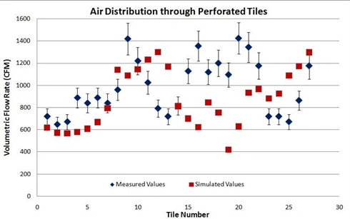
Figure 4
Air flow distribution through perforated floor tiles
In a revised CoolSim model, these obstructions were added to the supply plenum, as done for each tile in the room, identified by number, with numbers corresponding to the letters referenced in Figure 1 in Table 3.
As can be seen, the simulated and measured values for most of the perforated tiles are not in very good agreement, with error that ranges from less than 1% to about 60%. The worst agreement appears to be for Tiles 12 – 21 (L through U), with the exception of Tile 14 (N). The simulation overpredicts the flow in the region shown in Figure 5. The revised predictions for airflow distribution were in much better agreement overall with the measurements, as shown in Figure 6. The average absolute error dropped by 8 points. It was believed by the team that had additional complexity been added to the underflow region, the predicted distribution would be in even better agreement with measurements.
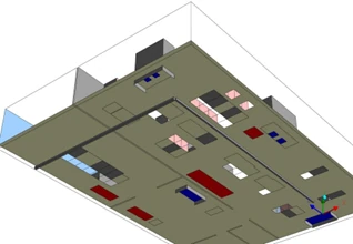
Figure 5
Pipes added to the plenum as underfloor obstructions
Another way of examining the role of underfloor obstructions is to compare the trajectories of the supply air with and without them. Pathline plots are used for this purpose. They represent the paths taken by imaginary “fluid particles” and can be colored by any variable. In Figure 7, the pathline plots in the supply plenum, colored by velocity magnitude, are compared for the case without (left) and with (right) underfloor obstructions. Clearly, even the addition of two relatively small objects can have a significant impact on the flowfield, and hence, the airflow distribution through the perforated tiles.
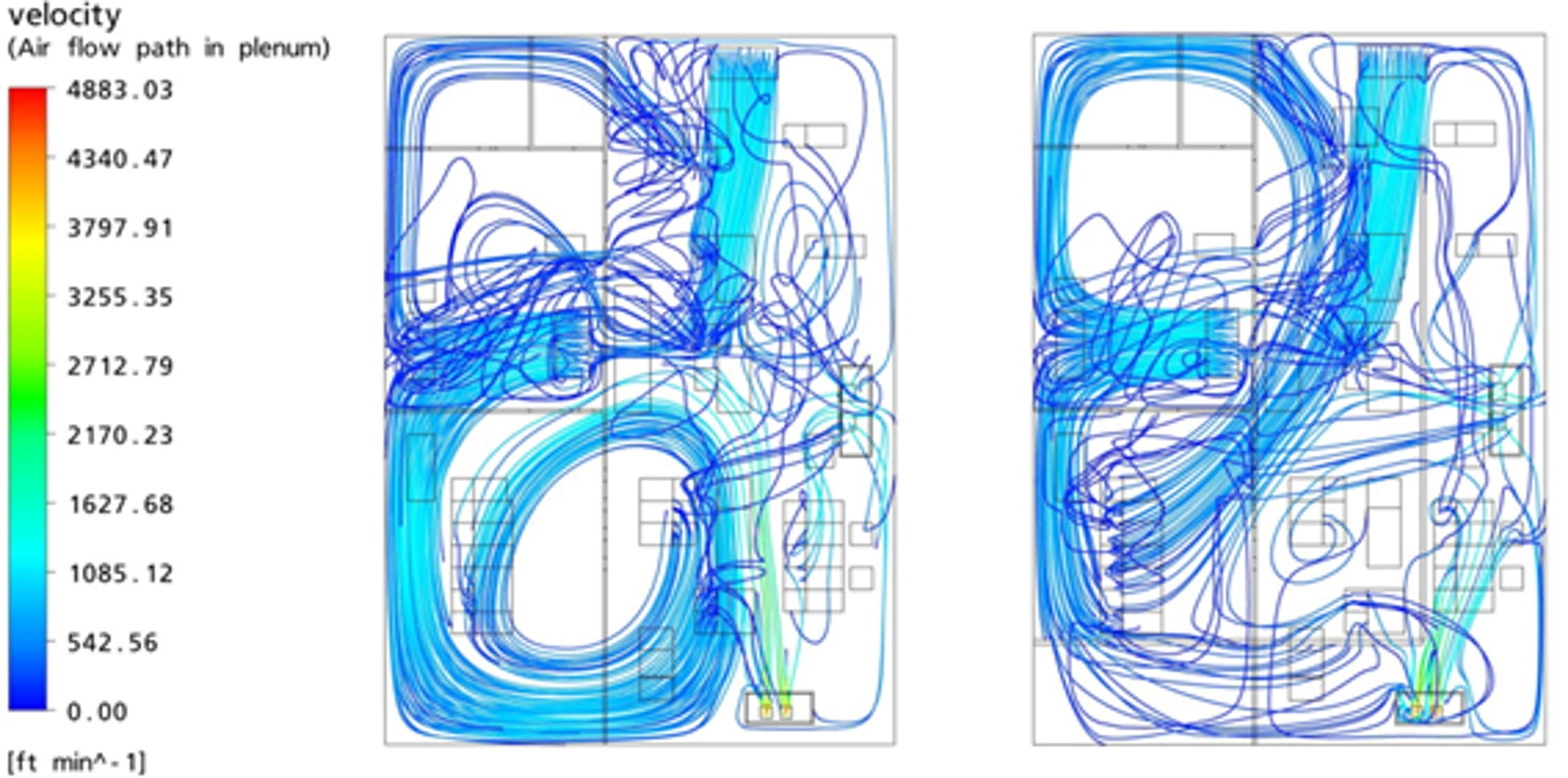
Figure 7
Supply plenum pathlines without (left) and with (right) underfloor pipes
Once the predicted airflow correlated adequately with measurements, comparisons of the simulated and measured rack inlet and exit temperatures were performed. In Figure 8 the inlet temperatures are shown to be in good agreement with data, with an overall average error of 13%.
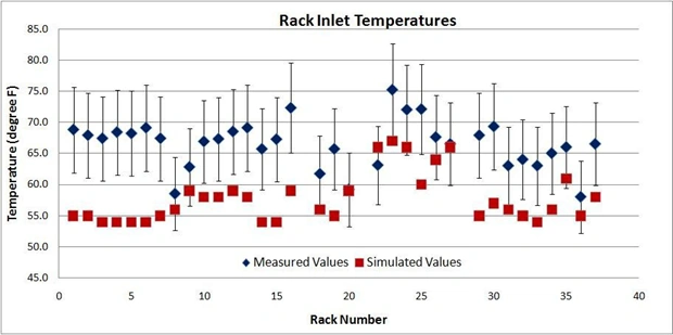
Figure 8
Rack inlet temperatures
The most consistent error in the rack inlet temperatures was for the row located in Operations Room 3, housing Racks 1 through 7 and in Operations Room 2, for Racks 29 through 34. For all of these racks, the simulation underpredicts the inlet temperatures. The airflow through the tiles in Room 1 is in good agreement with measurements and is underpredicted for the tiles servicing Racks 29 through 34. This means that the likely reason for the underpredicted temperatures is the assumption that the CRACs are operating with maximum cooling capacity. The air being supplied by the CRACs in the model is too cold. Even if one CRAC is not capable of meeting its cooling target, its warmer supply air could mix with the other supply air in the plenum and impact the rack inlet temperatures. It is also possible that additional under floor obstructions contribute to this discrepancy, since they would contribute to thermal mixing and air distribution.
A comparison of rack exit (outlet) temperatures was also performed, and the results are presented in Figure 9. The exit temperature error averaged 10%. For Racks 1 through 7 and 29 through 34, the exit temperatures are less than the measured values, as was true for the inlet temperatures on these racks.
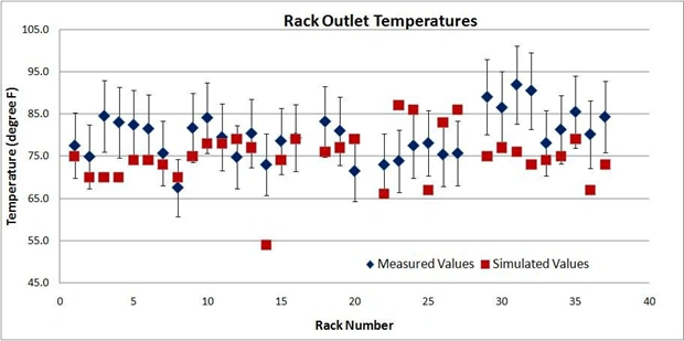
Figure 9
Rack outlet temperatures
This enforces the suggestion that the error is due to the supply air being too cold. In some cases, CoolSim underpredicts the rack inlet temperature yet overpredicts the rack outlet temperature. Rack 23 is one example, and it can be concluded that the rack heat load in the model was assumed to be too high. For Rack 22, on the other hand, the inlet temperature prediction was too high and the exit temperature prediction too low, suggesting that the rack heat load was assumed to be too low.
In CoolSim, the “cooling capacity” type of boundary condition for CRACs removes only as much heat as needed to maintain a user-specified thermostat temperature at the return. The cooling capacity that is set by the user is simply the maximum heat that the unit can remove from the return air. When the manufacturer’s cooling capacities were used in the simulation, the actual heat removal was reported to be less than these values for all CRACs in the data center. Even so, an additional simulation was performed to examine the effect of aging on two of the units. CRAC Unit 3 (about 10 years old) was set to operate at 80% of its rated value and CRAC Unit 4 (about 20 years old) was set to operate at 70%. CRAC Units 1 and 2 were not changed. The impact of these reductions on the rack inlet temperatures can be seen in Figure 10, where the simulated values using the full and reduced CRAC cooling capacities are shown.
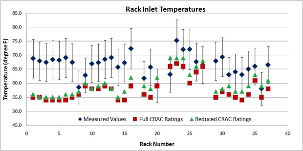
Figure 10
Rack inlet temperatures computed using full and reduced cooling capacity ratings on CRAC Units 3 and 4
These results show a small increase in the predicted inlet temperatures, with the overall error dropping to 11%. The increase is small because the CRACs do not need to operate at their peaks, given the cooling demands of the room. Even so, the units that operate at their full ratings need to work harder when the other units operate at reduced levels. In Table 4, the actual heat removed by each CRAC is compared to the cooling capacity boundary condition for the two scenarios. When Units 3 and 4 operate at reduced levels, Units 1 and 2 operate at increased levels. The division of labor changes because the diminished cooling capacity of Unit 3 is smaller than the heat it was called upon to remove when running at maximum value.
| Unit | Cooling Capacity (kW) | Heat Removal (kW) |
|---|---|---|
| 1 | Run 1: 35.00 Run 2: 35.00 | Run 1: 21.67 Run 2: 26.51 |
| 2 | Run 1: 35.00 Run 2: 35.00 | Run 1: 15.55 Run 2: 18.00 |
| 3 | Run 1: 35.00 Run 2: 27.81 | Run 1: 28.37 Run 2: 26.66 |
| 4 | Run 1: 51.00 Run 2: 35.78 | Run 1: 34.40 Run 2: 28.28 |
Table 4
Cooling capacity boundary conditions and resulting heat removal for CRACs modeled with their full ratings and with reduced ratings on Units 3 (80%) and 4 (70%)
This exercise identifies Unit 3 as a potential weakness in the data center. It is old, yet needs to operate at close to its maximum rated value. Even the newest CRACS, Units 1 and 2, could be operating at reduced levels. A simulation was performed in which all of the units were derated by 30%, and this reduced the error for Racks 1 through 7 by 30% compared to the fully rated case and the overall error for the inlet temperatures by 40% (from 13% to 8%).
Recommendations for Improved Efficiency
Once the validity of the model was established, the simulation results were studied to see if recommendations could be made to improve the data center’s efficiency. A number of key problem areas were found.
First, as shown above, the cooling load was not evenly distributed between the four air conditioning units, and Unit 3 may be overtaxed. By balancing the load among the CRACs, the data center would be better prepared for a potential failure of one of them.
Another common problem that was observed is that some of the cold air coming out of the floor tiles travels directly to the CRAC returns without ever passing through the racks. This phenomenon is known as short-circuiting and is shown in Figure 11 below.
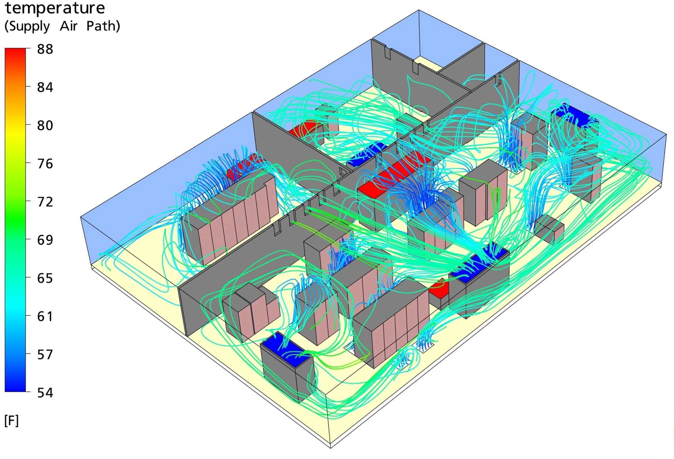
Figure 11
Short-circuiting of the supply air to the CRAC returns (royal blue)
Here, supply pathlines trace the trajectories of air from their entry into the room at the perforated floor tiles to their exit points, which should be at the rack inlets. The image shows that some of the trajectories go directly to the CRAC returns (shown in blue) in Operations Room 2. While short-circuiting in general reduced efficiency, some is to be expected in the UNH Data Center, however, because there is an abundance of supply air. As IT equipment is added to the facility in the future, it will be important to make sure that short-circuiting does not keep the available supply air from reaching the racks.
Finally, CRAC 2 in Operations Room 1 is located in an area with virtually no heat load other than a power supply. By either removing the surrounding walls or relocating the unit, it could be more effectively utilized. These main results, as well as some smaller details, are now providing the foundation for the alternative designs.
Conclusions and Future Work
During the past four months, the UNH data center has been studied and the behavior of the system analyzed. The design team conducted extensive research to develop an understanding of the causes behind the current data center operating characteristics. At this point, the system has been effectively modeled, so the dynamics of the system are well understood. The model can now be used to test design alternatives to see if the efficiency of the facility can be improved.
A few obstacles were encountered during the first phase of this project. First, the task of obtaining measurements from the existing data center was challenging due to time constraints and instrument limitations. For future measurements, additional velocity and temperature transducers should be purchased. Furthermore, a velometer would provide an improved method of capturing the true volume flow rate from the perforated floor tiles, compared to the current method, which is somewhat crude. During the creation of the CFD model, approximations were made when specifying the heat loads of the racks. The original heat loads were based on technical specifications supplied by the manufacturers; however these values represented worst case scenarios (with the highest possible heat loads) and were not necessarily representative of the real system. Using the room measurements as a guide, the team was able to adjust the heat loads of the racks until valid results were achieved. Through this process, the team developed a sense of engineering judgment that will be useful in later aspects of the project. The next focus of the project will be on developing system improvements and modeling the increase in thermal load anticipated for the next couple of years. All of these results will be presented to the director of UNH Data Services for review.
Acknowledgements
The UNH design team would like to thank a number of people who made this project possible. We would like to recognize the management team at the UNH Data Center, for their enthusiasm and cooperation throughout this project, and for allowing us to spend significant time in the data center gathering data. We would like to thank Professor John McHugh for acting as an advisor to the team, and for his assistance with the mathematical model of the system. Additionally, we would like to give a special thanks to the support staff at Applied Math Modeling Inc., for the use of their modeling tools, and for their valued support throughout the semester.