WP105: CRAC Thermal Boundary Condition Options in CoolSim
Introduction
Numerical simulations of data centers require models for the heat generating equipment, such as racks and power density units, and for the computer room air conditioners, or CRACs. The calculation is considered complete, or converged, when a heat balance is achieved. That is, the heat generated by the equipment in the room closely matches the heat removed by the cooling units. Any difference leaves or enters the room through the walls, based on the temperature of the adjacent rooms and resistance of the wall material.
While the CRACs need to remove the heat generated in the room, they can be directed to do so in a variety of ways. For example, the supply temperature can be set to an arbitrary value or the temperature drop across the CRAC can be prescribed. In CoolSim, four different cooling methods are available and the purpose of this paper is to illustrate how each works and when it is best applied. The cooling specifications, along with the air flow rate through the unit, are collectively referred to as the CRAC boundary conditions.
A CRAC in CoolSim consists of three objects: a hollow block (inside which the fluid flow is not computed) and two fans, one for the return air and one for the supply. This group of objects is used for all types of CRACS: downflow, upflow, in-row, and overhead cooling units. The shape of the block and locations of the supplies and returns are all that differ. The supply and return fans are set up so that they have equal total flow rates. That is, if there are two supplies but only one return, the sum of the supply flow rates equals the return flow rate. The return air temperature is that of the approaching air, while the supply air temperature is set according to the thermal boundary condition in use
The amount of heat that a CRAC removes from the air depends on three things: the return temperature, the supply temperature, and the flow rate of air through the unit. The following relationship is used to describe this dependence:
\[\dot{Q}=\dot{m}\,c_p\,\Delta T\]where:
- \(\dot{Q}\) is heat removed
- \(\dot{m}\) is mass flow rate of air
- \(c_p\) is specific heat of air
- \(T_R\) is return temperature
- \(T_S\) is supply temperature
In addition to the flow rate, the boundary condition options in CoolSim allow one or more of these variables to be set. The four methods: supply temperature, temperature drop, cooling capacity, and performance data, are described below. For each case, the summary report, returned at the completion of the calculation, provides values for all of these variables for each CRAC in the room.
Test Case Description
A simple test case is used to illustrate the different types of thermal boundary conditions. A small raised-floor data center is 20 ft x 10 ft with a 1.5 ft supply plenum and a 10 ft room height. A single row of six 4 kW racks is positioned next to a row of perforated tiles with a 25% open area. The room is cooled by a User-Defined CRAC with an air flow rate of 4000 CFM. The room geometry is shown in plan view and 3D rendering in Figure 1.
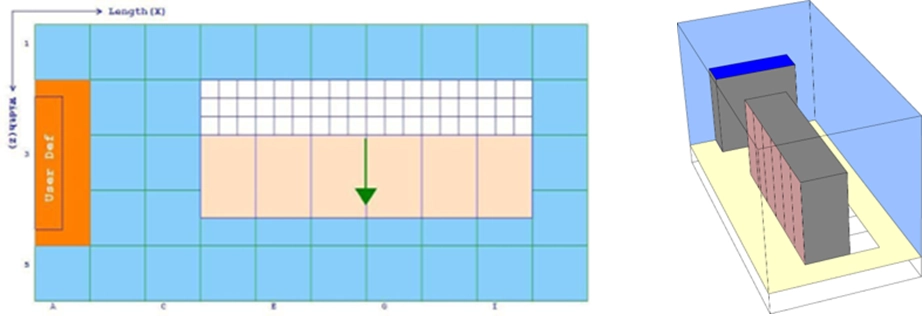
Figure 1
Plan view (left) and 3D view (right) of the sample test case, showing the CRAC, row of racks, and perforated tiles
Supply Temperature
Perhaps the most straightforward method of setting up a CRAC is to specify its supply temperature. This boundary condition is appropriate if the CRAC supply temperature is known. For non-raised floor models in which ducts and diffusers are used to distribute the cooling air, the supply temperature is the only boundary condition that can be applied to the CRACs.
To set up the supply temperature, simply choose this option from the Cooling Specifications list in the Specifications tab when the CRAC is selected (Figure 2).
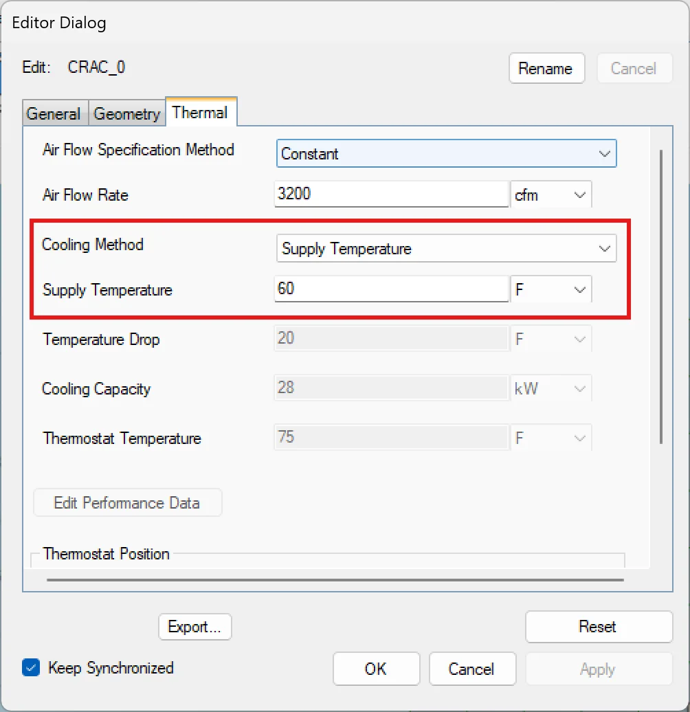
Figure 2
Choosing the Supply Temperature boundary condition
The summary report, returned after the calculation is complete, reports the average supply and return temperature, along with the heat removed by the unit (Table 1).
| Supply Temperature (°F) | Avg. Return Temperature (°F) | Avg. Supply Temperature (°F) | Supply Flow Rate (CFM) | Heat Removal (kW) |
|---|---|---|---|---|
| 60 | 70 | 60 | 4000 | 23.72 |
Table 1
The simulation results for the Supply Temperature boundary condition, including average supply and return temperature and heat removal
Not surprisingly, the reported supply temperature is exactly the same as the preset value.
Temperature Drop
When the temperature drop boundary condition is chosen, the thermostat temperature also needs to be set (Figure 3).
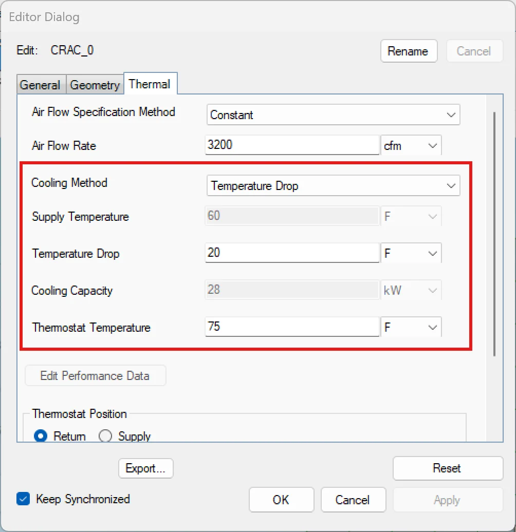
Figure 3
Setting the Temperature Drop across the CRAC also requires setting a thermostat temperature
The thermostat temperature is the desired room temperature in the vicinity of the CRAC. During the calculation, the average return temperature will continually be computed. If it is higher than the thermostat temperature, the supply temperature will be reduced with the constraint that the temperature drop target be met. If the return temperature is too low, the supply temperature will be increased in the same manner. Thus two simultaneous goals are being met when this boundary condition is used.
In Table 2, the results for the sample case are shown when a temperature drop of 20°F is specified for a range of thermostat temperatures.
| Thermostat Temperature (°F) | Avg. Return Temperature (°F) | Avg. Supply Temperature (°F) | Supply Flow Rate (CFM) | Heat Removal (kW) | Temperature Drop (°F) | Return vs. Thermostat Temperature Error (%) |
|---|---|---|---|---|---|---|
| 60 | 60 | 40 | 3985 | 26.75 | 20 | 0 |
| 65 | 64 | 46 | 4000 | 24.29 | 18 | 1.54 |
| 70 | 69 | 51 | 4000 | 24.12 | 18 | 1.43 |
| 75 | 74 | 55 | 4000 | 23.95 | 19 | 1.33 |
| 80 | 78 | 60 | 4000 | 23.78 | 18 | 2.50 |
| 85 | 83 | 65 | 4000 | 23.61 | 18 | 2.35 |
| 90 | 88 | 69 | 4000 | 23.44 | 19 | 2.22 |
Table 2
Results of the Temperature Drop boundary condition for a drop of 20°F and a range of thermostat temperature settings
In one case, the return temperature is identical to the thermostat temperature and the temperature drop is exactly 20°F. In the remaining cases, the return temperature is within 2°F of the thermostat temperature and the temperature drop is within 2°F of the target value. The maximum error is 2.5%. These results demonstrate that the temperature drop boundary condition is a reliable one to use if the difference between the room and supply temperature is known.
Cooling Capacity
The cooling capacity boundary condition is best reserved for cases in which the anticipated heat removal by a CRAC is known ahead of time. For example, if it is known that a particular unit is operating at or near is rated capacity, the cooling capacity of the CRAC can be used as a boundary condition and the other parameters, such as supply and return temperature, will be computed. When setting the cooling capacity boundary condition, the thermostat temperature must also be set (Figure 4).
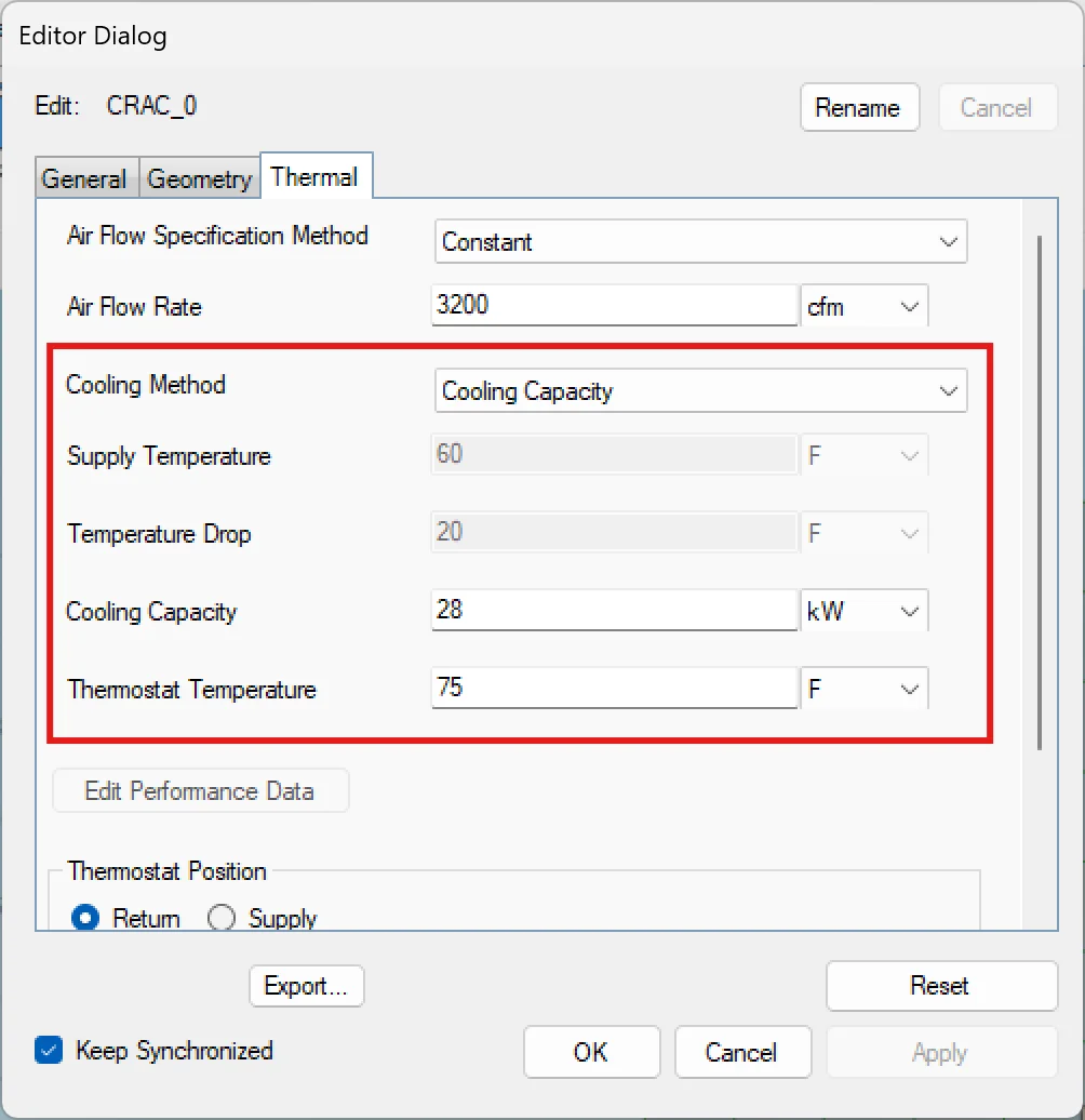
Figure 4
Choosing the Supply Temperature boundary condition
As with the temperature drop boundary condition, the solver will iterate on the supply temperature until the return temperature matches the preset thermostat temperature. The efficacy of this boundary condition is strongly dependent on how close the actual heat removal matches the cooling capacity set in the above panel. If the unit is operating a half steam, for example, the agreement between the return temperature and thermostat temperature will not be as close as if the unit operates nearer to its preset level. This is illustrated in Figure 5, where the return temperature is plotted against the cooling capacity for the test case, which carries a 24 kW heat load in the racks.
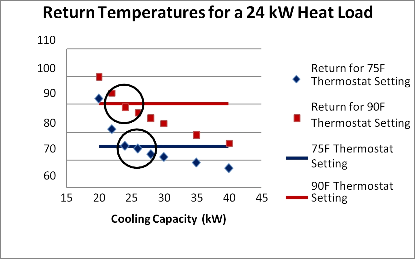
Figure 5
Return temperature as a function of cooling capacity for the test case with a heat load of 24 kW
Two thermostat settings are shown: 75°F and 90°F. The return temperature is above the thermostat temperature for cooling capacities below the heat load. This is partially due to the fact that the CRAC cannot meet the target thermostat temperature when the heat load in the room exceeds its capacity. When the specified cooling capacity is much greater than the heat load, the CRAC over-cools the space and the return temperature is below the thermostat temperature. It is only when the cooling capacity is close to the target heat removal of 24 kW (the circled areas) that the return and thermostat temperatures are in good agreement.
Performance Data
Performance data is available for a number of the library CRACs in CoolSim and is perhaps the most accurate way to capture the CRAC performance. The data consists of ordered pairs of heat removal and return temperature. That is, for a given return temperature a specified amount of heat is removed by the CRAC. A linear interpolation is done between the points. The CoolSim panel is shown in Figure 6, along with some of the data pairs in a 9-point sample.
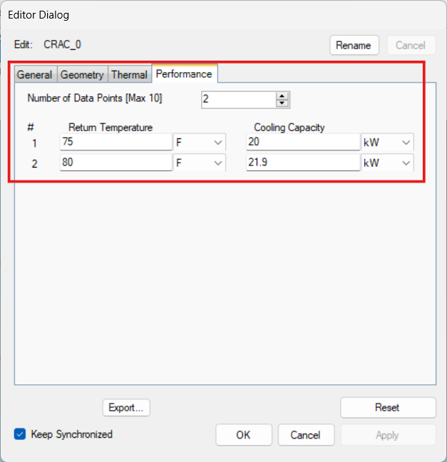
Figure 6: The performance data boundary condition uses ordered pairs of return temperature and cooling capacity
A thermostat setting is also shown in the panel, but this plays a different role than when the other boundary conditions are used. Here, the thermostat temperature marks the minimum temperature that the CRAC will allow for the return air. In this regime, the supply temperature is adjusted to ensure that the temperature does not drop below this value. To illustrate CRAC performance when this type of boundary condition is used, the performance curve shown in Table 3 is used for the simple test case, but the total heat load of the 6 racks is varied from 12 kW (below the minimum) to 42 kW (above the maximum).
| Return Temperature (°F) | Heat Removal (kW) |
|---|---|
| 60 | 18 |
| 65 | 21 |
| 70 | 24 |
| 75 | 27 |
| 80 | 30 |
| 85 | 33 |
| 90 | 36 |
| 95 | 36 |
| 100 | 36 |
Table 3
Performance data for the simple test case in which the total rack heat load is varied
The computed heat removal as a function of return temperature is shown in Figure 7. When the total heat load is below the minimum in the Table 3 data, the minimum (thermostat) temperature is the target for the return temperature. For total heat loads of 12 and 15 kW, the return temperatures are 59 and 60°F. For heat loads between 18 and 36 kW, the return temperatures closely match the performance data curve. Heat loads of 39 and 42 kW are above the maximum set forth in the data. To achieve a heat balance, the excess heat passes through the walls to the adjacent rooms, but the temperature in the room is nonetheless quite high. This effect is seen as heat removal saturation in Figure 7.
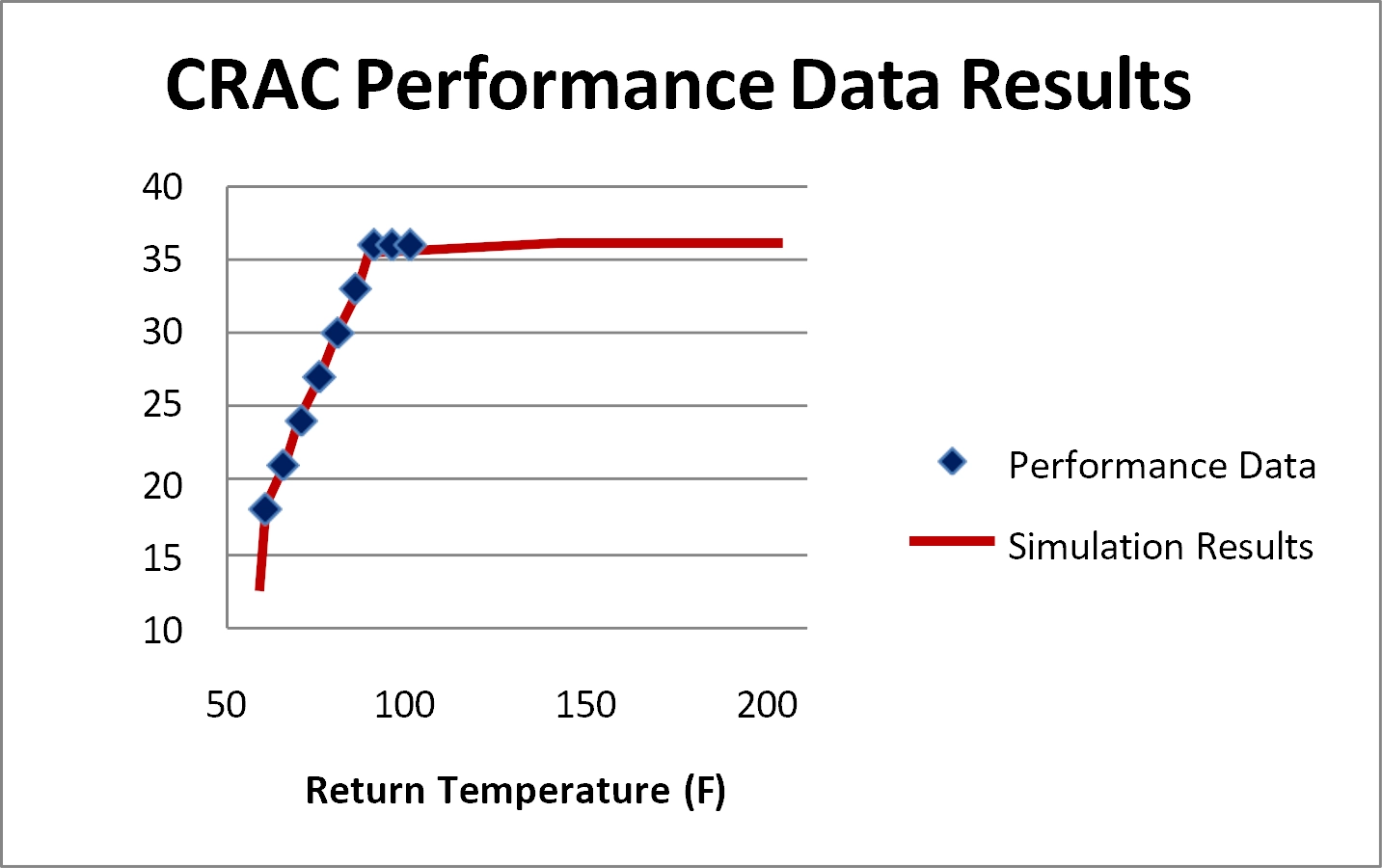
Figure 7
CRAC performance when ordered pairs of heat removal vs. return temperature are used as boundary conditions
While this boundary condition may not be the best choice for performance outside the data limits, it is certainly the most accurate way to describe the CRAC within the limits.
Summary
CoolSim offers four methods for modeling CRAC thermal boundary conditions.
- Supply Temperature is the best choice if the value is known from measurements
- Temperature Drop depends on the thermostat temperature, and is often used as a target condition
- Cooling Capacity is best if the approximate heat removal is known ahead of time. Since this is rarely the case, this option should be used with care.
- Performance Data is the most accurate, and many CRAC manufacturers make this data available to their customers
No matter which cooling method is used however, the report provides a comprehensive summary of the CRAC performance.