WP106: Transient CRAC Failure Analysis
Introduction
One of the largest concerns facing data center facility managers is the loss of power, particularly in the middle of the night when staff may not be present. The IT equipment is usually protected by uninterruptable power supplies (UPSs), which switch to battery power as soon as the building power goes down. The cooling equipment, however, does not usually have backup power unless generators are installed with automatic starters. Depending on the size of the data center, generators may be nonexistent or slow to come up to speed. Thus while the UPS systems keep the IT equipment (and subsequent heat release) functioning at its pre-power-failure level, the cooling units may experience a lag or abrupt end in their operation. Accompanying any loss of cooling will be an increase in room temperature that can bring a disastrous end to the equipment, ongoing processes, and data. The question on facility managers’ minds, therefore, is “How much time will elapse before this point is reached?"
One way of estimating the time to failure is through computational fluid dynamics, or CFD.
CFD has been used for decades to simulate the flow and heat transfer in a variety of settings, including interior spaces with heat sources and losses.
While the simplest type of CFD analysis results in a steady-state solution, an estimation of the time to failure can also be done using a transient analysis that begins with the steady-state flow field in a normally operating data center.
In this paper, CoolSim software from Applied Math Modeling Inc. is used to perform a steadystate simulation of a typical data center.
The model is then exported to ANSYS Airpak software, where some or all of the cooling units are disabled.
Using the steady-state results as initial conditions, transient calculations are performed with temperature sensors at several locations in the room.
The increase in temperature following the loss of cooling power is then tracked, indicating the trouble spots and the rate of increase of temperature at those (and other) locations.
Problem Description
An 1800 sq.ft. raised-floor data center is used as an example. The room is 10 ft high with an 18 in supply plenum. The IT equipment is distributed in twelve rows of racks, some of which contain gaps between the servers (Figure 1).
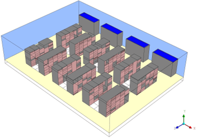
Figure 1
The geometry of the raised-floor data center showing racks of IT equipment (pink faces) and CRACs (blue tops)
Each row contains five racks and with a total heat load of 315.25 kW in the room, the racks have an average heat load of 5.25 kW. The heat density in the room is 174 W/ sq.ft. Each of the four CRACs along one side of the room delivers 60°F supply temperature at 12,000 CFM. The combined CRAC flowrate is 18% above the total airflow demand from the IT equipment. Two rows of Tate GrateAire-24 tiles (56% open) line the cold aisles.
Steady-State Results
As a first step, a steady-state calculation is performed using CoolSim to obtain a picture of the data center under normal operating conditions. For the IT equipment, the most important result is the maximum inlet temperature on the racks (Figure 2).
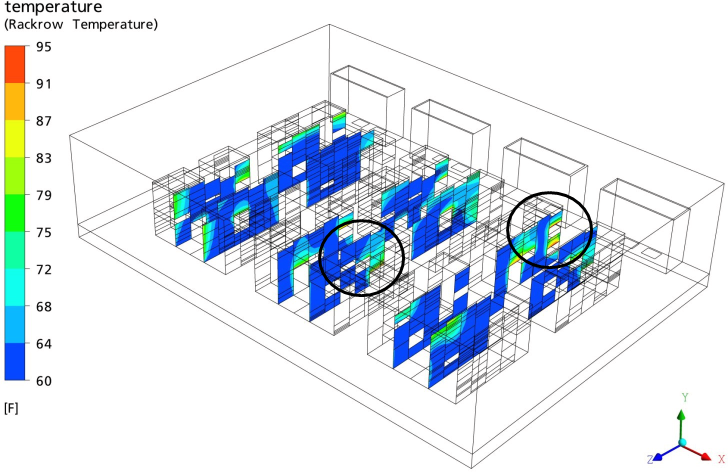
Figure 2
Contours of rack inlet temperatures for the steady-state run showing the locations of the four server with maximum rack inlet temperatures exceeding the ASHRAE allowed values
The 2008 ASHRAE guidelines recommend a maximum inlet temperature of 80.6°F, but publish an allowed maximum value of 90°F. Of the 400 servers in the room, 27 are above the recommended temperature maximum and 4 are above the allowed temperature maximum, with values of 90°F, 90°F, 93°F, and 94°F. These four servers are in the two circled regions in Figure 2. Their average inlet temperatures are all below the acceptable limit, however, with values of 82°F, 86°F, 85°F, and 83°F, respectively. This is acceptable performance for the data center as a whole, but certainly not optimal. In ideal conditions, all of the racks would have maximum inlet temperatures below the recommended maximum value.
In Figure 3, temperature contours at a height of 3 ft off the floor are shown.
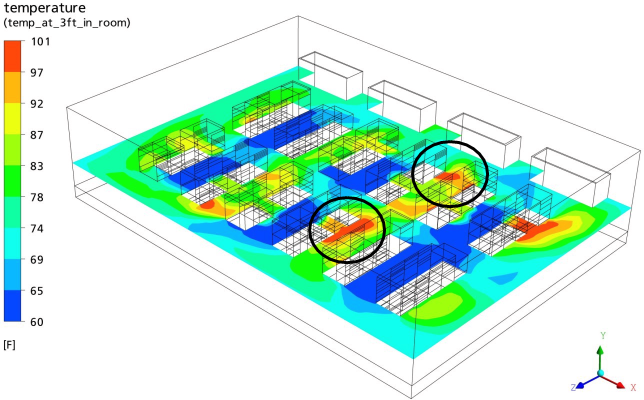
Figure 3
Temperatures 3 ft above the floor for the steady-state conditions; some of the hot exhaust air in the circled areas is entrainedby nearby server inlets
Several high temperature regions can be seen on the exhaust sides of the racks. These produce high room temperatures and are of particular concern in this data center where there are gaps between the equipment in the racks. In Figure 4, pathlines of return air in one of these regions are shown to leak through gaps between the equipment and heat the supply air to unsafe temperatures.
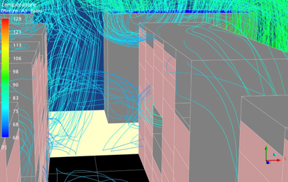
Figure 4
Return air pathlines show the entrainment of exhaust air through gaps between the middle tile row
Steady-state conditions such as these provide helpful information in advance of a transient CRAC failure calculation, since probes can be positioned in the problem areas to track the increasing temperatures.
Transient Analysis
Partial Failure
The data center model, built in CoolSim, is exported to Airpak, where two transient calculations are performed. At the start of the first transient run, the two CRACs on the left side of the room (in plan view) are disabled.
That is, their fans are shut down and the CRACs are represented as hollow blocks with adiabatic boundary conditions on all sides. Because two CRACs continue to operate, this case represents a partial failure of the cooling system. Monitor points are created at four locations in the data center: two in hot aisles and two in cold aisles, as shown in Figure 5. The steady state data is used as the starting point and a transient calculation is performed for approximately two minutes following the CRAC failure. A time-step of 0.1 seconds is used and data is saved every 15 seconds.
That is, their fans are shut down and the CRACs are represented as hollow blocks with adiabatic boundary conditions on all sides. Because two CRACs continue to operate, this case represents a partial failure of the cooling system. Monitor points are created at four locations in the data center: two in hot aisles and two in cold aisles, as shown in Figure 5.
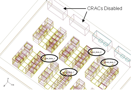
Figure 5
Two CRACs are disabled for the transient calculation and the temperatures at four monitor points (circled) are recorded
The steady-state data is used as the starting point and a transient calculation is performed for approximately two minutes following the CRAC failure. A time-step of 0.1 seconds is used and data is saved every 15 seconds.
The temperatures recorded at the monitor points are shown in Figure 6 during the first 2 minutes following the failure of the two CRACs.
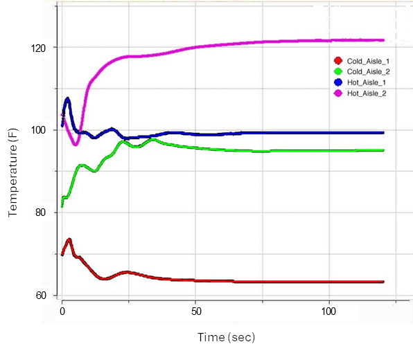
Figure 6
Temperatures at four monitor points during the transient caluclation of a partial cooling failure in the data center
The temperatures in all four locations change initially, but they soon stabilize at new values. One hot aisle temperature increases dramatically while the other increases but soonreturns to slightly below its initial value. One cold aisle temperature shows a marked increase while the other shows a decrease.
Taking a closer look, the point with the highest final temperature, Hot_Aisle_2, is closest to one of the working CRACs. When two of the CRACs are disabled, the air rushes out from the two working CRACs to fill the plenum, and the high speed air causes negative flow through some of the nearby perforated tiles. This effect, which is common in data centers, is shown in Figure 7, where the y-component of velocity on the top surface of the vent tiles is shown after two minutes.
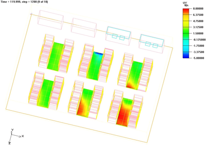
Figure 7
Contours of the veritcal (y) component of velocity are shown on the upper srufaces of the perforated tiles after two minutes. The central tile row shows flow entering the plenum in the region nearest the middle working CRAC
The velocity is negative in front of the servers that exhaust in the region of the point Hot_Aisle_2. This lack of supply air starves the servers, causing them to draw air from nearby rack exhausts instead. Contours of temperature on a plane 5ft above the floor, shown in Figure 8, further illustrate the resulting hot spots.
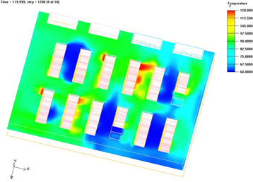
Figure 8
Temperature contours on a plane 5 ft above the floor, two minutes after the failure; the hotttest temperatures are in the hot aisles behind servers whose supply air is cut off by downdrafts into the plenum
One final point should be made regarding the partial failure mode represented here. In order to reach equilibrium with two CRACs shut off, the remaining two CRACs have to work harder so that an overall heat balance is achieved in the room. While these CRACs can operate above their rated cooling capacity in the model, they cannot do so in practice. This exercise therefore illustrates the changes to the flow and thermal patterns in the room, but the steady-state condition reached does not correspond to a situation that is sustainable.
Total Failure
The second failure scenario studied corresponds to the case where all four CRACs are suddenly disabled. All supply and return fans are removed from the CRACs, and only the blocks representing their housing remain. Because there is no mechanism in place for heat removal, this simulation will not reach steady-state. Instead, the temperature throughout the data center will continue to rise with time. In Figure 9, temperatures at the four monitor points are shown during the first minute.
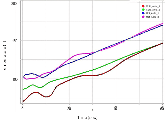
Figure 9
Temperatures at four monitor points following the failure of all four CRACs in the data center
The temperatures in both the hot and cold aisles fluctuate until 40 or 50 seconds, after which they increase at a steady rate, with the two cold aisle temperatures approaching the same value and the two hot aisle temperatures doing the same.
The rapid change in the temperatures in the room is illustrated in Figure 10, where four images represent the conditions at 30 second intervals. The minimum temperature is 60°F and the maximum is 200°F.
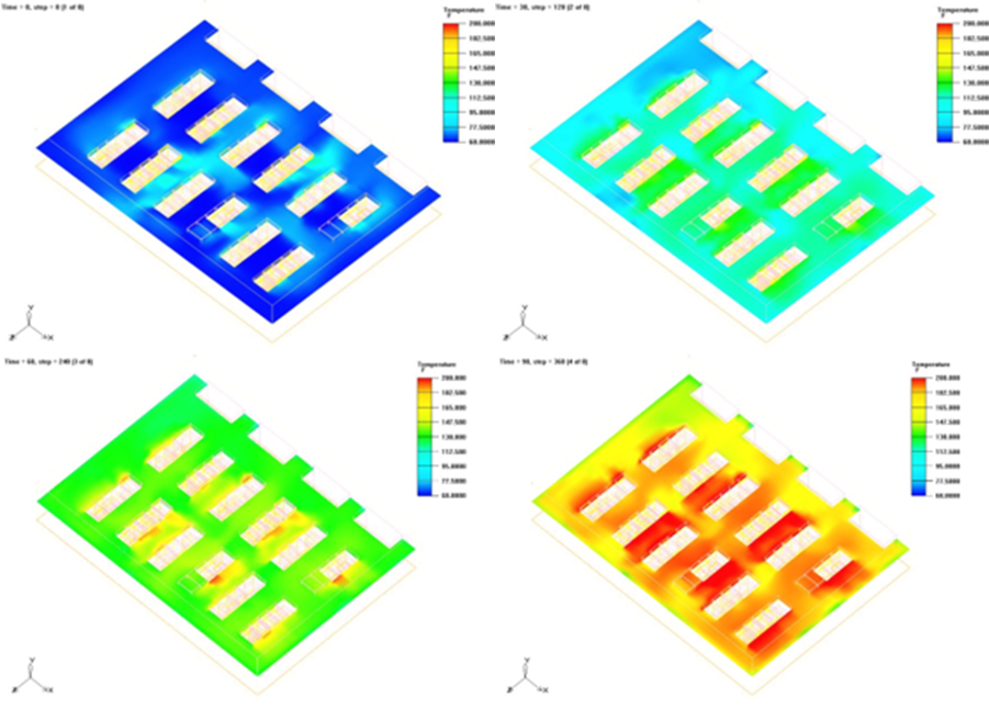
Figure 10
Contours of temperature on a plane 5 ft off the floor at times 0s (top-left), 30s (top-right), 60s (bottom-left), and 90s (bottom-right)
It is clear that in the case of a complete failure, there is very little time available before backup generators start up to continue cooling the data center. Otherwise, temperatures will reach catastrophic levels.
Summary
A data center modeled with server-level detail was used to perform two “what if” calculations in the case of CRAC failure. A steady-state calculation was done in CoolSim with all CRACs on. The results of this calculation pointed to areas in the room where the temperatures were highest and the equipment most vulnerable. The model was exported from CoolSim into Airpak, where two transient calculations were performed. When two CRACs were disabled, the room conditions reached a new equilibrium, but in order to achieve a heat balance within the room (numerically), the CRACs were required to remove more heat than they are rated to do. Gaps between servers in the racks, coupled with poor flow conditions near some of the perforated tiles led to the entrainment of exhaust air into the server inlets, which worsened the conditions in certain areas.When all four CRACs were disabled, the conditions in the room deteriorated rapidly. Such an exercise is useful in planning for back-up power generation needs in the case of a complete power outage.